R computations with normal distributions
There are various R functions which are useful for computation with normal distributions, such as pnorm( ), qnorm( ), and dnorm( ).
The pnorm( ) function gives the cumulative distribution function, and the alphabet ‘p’ stands for probability. The qnorm( ) is for quantiles whilst the dnorm( ) function, the density.
Let’s use the statistical notation for normal distribution: X ~ N(µ,sigma2). We shall illustrate the usage of these R functions.
R function pnorm( )
For example, let X ~ N(8,4), then
- the probability P(X < 2) can be computed via pnorm( ) in several different ways:
> pnorm(2,mean=8,sd=2) #P(X<=2) in N(8,4)
[1] 0.001349898
> pnorm(2,8,2) #P(X<=2) in N(8,4) simplified
[1] 0.001349898
- the probability P(X < 1.96) for x ~ N(8,4) by R language is:
> pnorm(1.96,8,2) #P(X<=1.96) in N(8,4)
[1] 0.001263873
Remember that for f(1.96) = 0.975 and f(1.645) = 0.950, respectively from the statistics table, the R gives us the same answers:
> pnorm(1.96,0,1) #P(X<=1.96) in N(0,1)
[1] 0.9750021
> pnorm(1.645,0,1) #P(X<=1.645) in N(0,1)
[1] 0.9500151
> pnorm(1.645) #P(X<=1.645) in N(0,1) simplified
[1] 0.9500151
>
And, when P(X < -1.645), the R result indicates the area on the left hand side of the normal distribution curve:
> pnorm(-1.645) #P(X<=-1.645) in N(0,1) simplified
[1] 0.04998491
>
R function qnorm( )
In layman’s language, a quantile is where a series of sample data is sub-divided into equal proportions. In statistics, we divide a probability distribution into areas of equal probability. The simplest division that can be envisioned is into two equal halves, i.e., 50%.
The R function: qnorm( ) is used to compute the quantiles for the standard normal distribution using its density function f.
> qnorm(0.95) #95.0% quantile of N(0,1)
[1] 1.644854
> qnorm(0.975) #97.5% quantile of N(0,1)
[1] 1.959964
R function dnorm( )
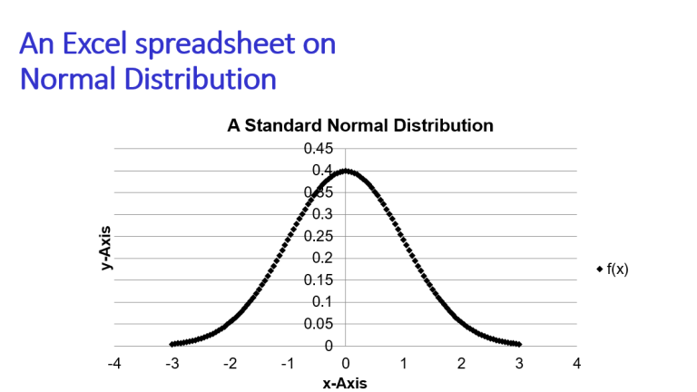
The density of a Gaussian formulae for normal distribution can be shown to be close to 0.4 when x = 0.
The R function dnorm(0) indeed gives the same result as below:
> dnorm(0) # Density of N(0,1) evaluated at x= 0
[1] 0.3989423
>
Further remarks
Like pnorm( ), the functions qnorm( ) and dnorm( ) can also be used for normal distributions with non-zero mean and non-zero standard deviation or variance, simply by supplying the mean and standard deviation as extra arguments.
For example, for the N(8,4) distribution, the results are self-explanatory:
> qnorm(0.975,8,2) # 97.5% quantile of N(8,4)
[1] 11.91993
> dnorm(1,8,2) #Density of N(8,4) at x=1
[1] 0.0004363413
> dnorm(4,8,2) #Density of N(8,4) at x=4
[1] 0.02699548
>
