
The equations (7) and (8) stated in the previous Part 1 article revealed an important message. That is when the measured value of y is closer to the mean value of y, the confidence limit approaches to a minimum value. Hence, in practice, a calibration experiment of this type will give the most precise results when the measured instrument signal corresponds to a point close to the centroid of the regression line.
This implies that we should always aim to prepare a calibration curve with a range that can effectively measure the analyte of sample solution nearer to its regression line central for better precision. This can be illustrated in the following worked example.
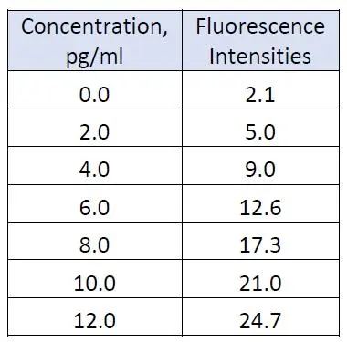
A series of standard aqueous solutions of fluorescein was used to calibrate a fluorescence spectrometer. The following fluorescence intensities (in arbitrary units) were obtained:

The least-squares regression equation was found to be y = 1.518 + 1.930x and its calibration graph plotted in Figure 1 is shown below:

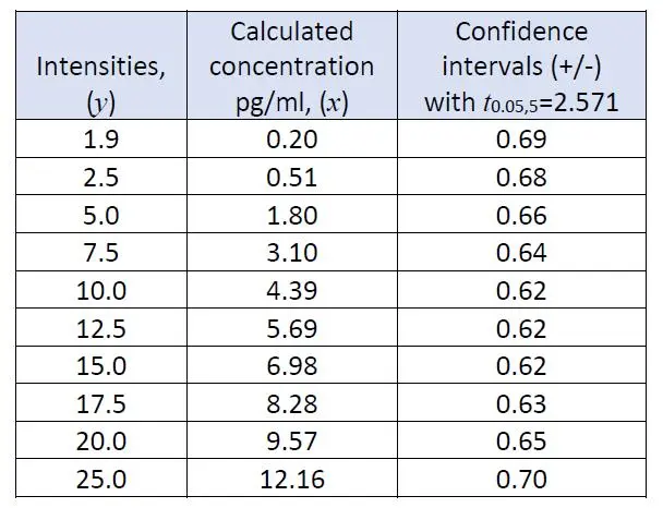
The important parameter for estimating the confidence intervals, i.e. standard error of y in x, sy/xwas found to be 0.433, with the number of points, n as 7. The concentrations in terms of x-values are easily calculated using the regression equation by substituting various intensities y-values, and also their corresponding confidence intervals using equation (7) as follows:

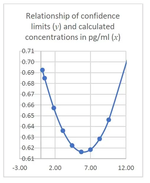
The changes of magnitude in confidence intervals against the calculated concentrations can be visualized by the following Figures 2 and 3:


It is thus obvious from both graphs that the confidence intervals become narrowest (+/- 0.62 pg/ml) at the centroid of the calibration curve, indicating a better measurement precision at this point.
An approach to improve the confidence limits in this calibration experiment is by increasing n, the number of calibration points on the regression line. Another way is by making more than one measurement of y-values, as using equation (8) with R greater than 1. Of course, we need to weigh the underlying benefits if we are to make too many replicate measurements (assuming that sufficient sample is available) or increasing the number of calibration points as compared with the additional costs, and time involved.
To determine the concentration of copper in treated mine waste water samples by atomic absorption spectrometry, we can prepare a series of aqueous solutions containing a pure copper salt to calibrate the spectrometer and then use the resulting calibration graph in the determination of the copper in the test samples.
This approach is valid only if a pure aqueous solution of copper and a waste water sample containing the same concentration of copper give the similar absorbance values. In other words, by doing so we are assuming that there is no reduction or enhancement of the copper absorbance signal by other constituents present in the test sample. In many areas of analysis, this assumption is not always true. Matrix effect can have a significant influence to the final answer, even with methods such as plasma spectrometry (say ICP-AES) which is widely known for being relatively free from interferences.
There can be so-called proportional effects as these effects are normally proportional to the analyte signal, resulting in a change of the slope of the calibration curve.
One way to overcome this is to prepare the calibration standards in a matrix that is similar to the test sample but free of the targeted analyte, by adding known amounts of a copper salt to it in this discussion. However, in practice, this matrix matching approach is not practical. It will not eliminate matrix effects that differ in magnitude from one sample to another, and it may not be possible even to obtain a sample of the copper mine waste water matrix that contains no such analyte.
So, a better solution to this problem is that all the analytical measurements, including the establishment of the calibration graph, must in some way to be performed using the sample itself. Hence, the method of standard additions is proposed. It is widely practiced in atomic-absorption and emission spectrometry, and has also been applied in electrochemical analysis and many other areas.
This method of standard additions suggests to take six or more equal volumes of the sample solution, ‘spike’ them individually with known and different amounts of the analyte, and dilute all to the same volume. The instrument signals are then determined for all these standard solutions and the results are plotted as a linear calibration graph which has the signals plotted on the y-axis with its x-axis graduated in terms of the amounts of analyte added (either as an absolute weight or as a concentration).
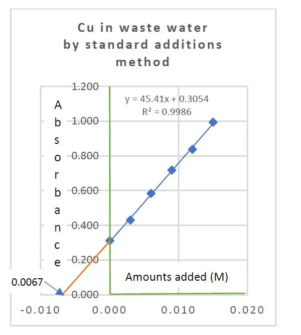
When this linear regression is extrapolated to the point on the x-axis at which y = 0, we get a negative intercept on the x-axis which corresponds to the amount of the analyte in the test sample. So, when the linear calibration equation is expressed in the form of y = a + bx, where a is the y-intercept when x = 0, and b, the slope or gradient of the linear curve, simple geometry shows that the expected amount of the analyte in the test sample, xE, is given by a/b in absolute term, which is the ratio of the intercept and the slope of the regression line.
Since both a and b are subject to error, the calculated concentration is clearly subject to error as well. However, as this concentration is not predicted from a single measured value of y, the formula for the standard deviation, sxE of the sample analyte from the extrapolated x-value, xE is as follows:

where sy/x is the standard error of y on x, and n, the number of points plotted on the regression. The standard error of y on x, sy/x of the linear regression is given by equation:

where yexp,i is the instrument signal value observed for standard concentration xi, and ycal,i, the ‘fitted’ yi-value calculated from the linear regression equation for xi value. This equation has made some important assumptions that the y-values obtained have a normal (Gaussian) error distribution and that the magnitude of the random errors in the y-values is independent of the analyte concentration (i.e. x-values).
Subsequently, we need to determine the confidence limits for xE as xE + t(n-2).sxE at alpha (a) error of 0.05 or 95% confidence. Increasing the value of n surely improves the precision of the estimated concentration. In general, at least six points should be used in a standard-additions experiment.
You may have noticed that the above equation differs slightly from the expression that is familiar in evaluating the standard deviation sx of an x-value given a known or measured y-value from a linear regression:

A worked example
The copper content in a sample of treated mining waste water was determined by FAAS with the method of standard additions. The following results were obtained:
Added Cu salt in moles/L 0.000, 0.0003, 0.006, 0.009, 0.012, 0.015
Absorbance recorded 0.312, 0.430, 0.584, 0.718, 0.838, 0.994
Let’s determine the concentration of copper level in the sample, and estimate the 95% confidence intervals for this concentration.
Apply the following equations for a, the y-intercept when x = 0, and b, the gradient or slope of the least-squares straight line expressed as y = a + bx:

These two equations yielded a = 45.4095 and b = 0.3054. The ratio a/b gave the expected copper concentration in the test sample as 0.0067 moles Cu per liter.

By further calculation, we have sy/x = 0.01048, sxE = 0.00028. Using Student’s t(6-2) critical value of 2.78, the confidence intervals are found to be 0.0067 M +/- 0.0008 M.
Although the method of standard additions is a good approach to cater for the common problem of matrix interference effects, it has certain disadvantages too:
You may also read our earlier article
https://consultglp.com/2018/12/23/std-additions-in-instrumental-calibration/

Category:
BASIC STATISTICS MEASUREMENT UNCERTAINITY
TAGGED WITH
Central limit theorem CONFIDENCE INTERVAL STUDENT'S T DISTRIBUTION