
Verifying the Excel’s one-factor ANOVA results
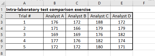
In a one-factor ANOVA (Analysis of Variance), we check the replicate results of each group under a sole factor. For example, we may be evaluating the performance of four analysts who have each been asked to perform replicate determinations of identical samples drawn from a population. Thus, the factor is “Analyst” of which we have four so-called “groups” – Analyst A, Analyst B, Analyst C and Analyst D. The test data are laid out in a matrix with the four groups of the factor in each column and the replicates (five replicates in this example) in each row, as shown in the following table:
We then use the ANOVA principal inferential statistic, the F-test, to decide whether differences between treatment’s mean values are real in the population, or simply due to random error in the sample analysis. The F-test studies the ratio of two estimates of the variance. In this case, we use the variance between groups, divided by the variance within groups.
The MS Excel installation files have included an add-in that performs several statistical analyses. It is called “Data Analysis” add-in. If you do not find it labelled in the Ribbon of your spreadsheet, you can make it available to Excel by installing it with your Excel 2016 version by clicking “File -> Options -> Add-ins -> Analysis ToolPak” and then pressing “Enter”. You should now find Data Analysis in the Analysis Group on your Excel’s Data tab.
We can then click the “Data Analysis” button to look for “Anova: Single Factor” entry and start its dialog box accordingly.
For the above set of data from Analysts A to D, the Excel’s Data Analysis gives the following outputs, and we shall then verify the outcomes through manual calculations based on the first principles:
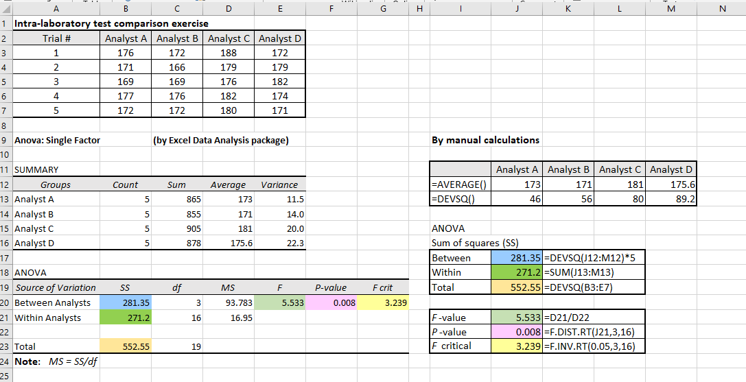
We know that variances are defined and calculated using the squared deviations of a single variable. In Excel, we can use the formula “=DEVSQ( )” to calculate each group of results. Also, we can use “=AVERAGE( )” function to calculate the individual mean of each Analyst.
In this univariate ANOVA example, we squared the deviation of a value from a mean, and the word “deviation” referred to the difference between each measurement result from the mean of the Analyst concerned.
The above figure shows the manual calculations using the Excel formulae agree very well with the Excel’s calculated data by its Data Analysis package. In words, we have:
Subsequently, we can also verify the Excel’s calculations of the F-value, P-value and the F critical value by using the various formulae as shown above.
We have normally set the level of significance at the P = 0.05 (or 5%), meaning that we are prepared to make a 5% error in rejecting the null hypothesis which states that there are no difference amongst the mean values of these four Analysts. The calculated P-value of 0.008 indicates that our risk of rejecting the null hypothesis is only at a low 0.8%.

Analysis of variance (ANOVA) is useful in laboratory data analysis for significance testing. It however, has certain assumptions that must be met for the technique to be used appropriately. Their assumptions are somewhat similar to those of regression because both linear regression and ANOVA are really just two ways of analysis the data that use the general linear model. Departures from these assumptions can seriously affect inferences made from the analysis of variance.
The assumptions are:
1. Appropriateness of data
The outcome variables should be continuous, measured at the interval or ratio level, and are unbounded or valid over a wide range. The factor (group variables) should be categorical (i.e. being an object such as Analyst, Laboratory, Temperature, etc.);
2. Randomness and independence
Each value of the outcome variable is independent of each other value to avoid biases. There should not have any influence of the data collected. That means the samples of the group under comparison must be randomly and independently drawn from the population.
3. Distribution
The continuous variable is approximately normally distributed within each group. This distribution of the continuous variable can be checked by creating a histogram and by a statistical test for normality such as the Anderson-Darling or the Kolmogorov-Smirnov. However, the one-way ANOVA F-test is fairly robust against departures from the normal distribution. As long as the distributions are not extremely different from a normal distribution, the level of significance of the ANOVA F-test is usually not greatly affected by lack of normality, particularly for large samples.
4. Homogeneity of variance
The variance of each of the groups should be approximately equal. This assumption is needed in order to combine or pool the variances within the groups into a single within-group source of variation SSW. The Levene statistic test can be used to check variance homogeneity. The null hypothesis is that the variance is homogeneous, so if the Levene statistic are not statistically significant (normally at alpha < 0.05), the variances are assumed to be sufficiently homogeneous to proceed in the data analysis.
Estimation of sampling and analytical uncertainties using Excel Data Analysis toolpak
https://consultglp.com/2018/08/22/a-worked-example-of-measurement-uncertainty-for-a-non-homogeneous-population/,we used the basic ANOVA principles to analyze the total chromium Cr data for the estimation of measurement uncertainty covering both sampling and analytical uncertainties….
A worked example of MU estimation on a non-homogeneous population
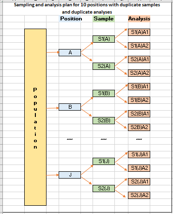
For sampling a non-homogeneous target population such as grain cargo, grainy materials or soil, random positions may be selected and split duplicate samples are taken with duplicate laboratory analysis carried out on each sample received. This approach will be able to address both sampling and analytical uncertainties at the same time…..
Data analysis for one factor analysis of variance ANOVA with an equal number of replicates for each ‘treatment’ is probably quicker and easier by using Excel’s traditional functions in the spreadsheet calculations.
One of the advantages is that the manual calculations return live worksheet functions rather than the static values returned by the Data Analysis Toolpak add-ins, so we can easily edit the underlying data and see immediately whether that makes sense or shows a difference to the outcome. On the other hand, we have to run the Data Analysis tool over again if we want to even change one value of the data.
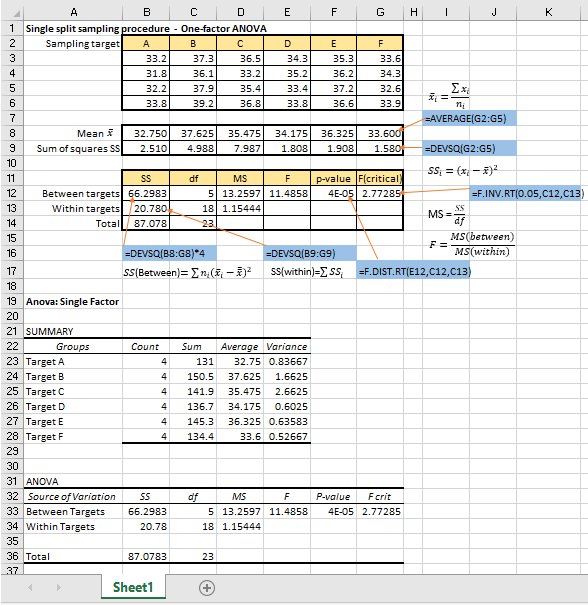
The following figure shows how simple it can be in analyzing a set of test data obtained from sampling at 6 different targets of a population with the laboratory samples analyzed in four replicates. The manual calculations have been verified by the Single Factor Tool in the Data Analysis add-in, as shown in the lower half of the figure.
With the variance results in the form of MS(between) and MS(within), we can proceed easily to estimate the measurement uncertainty as contributed by the sampling and analytical components.

A simple example of sampling uncertainty evaluation
In analytical chemistry, the test sample is usually only part of the system for which information is required. It is not possible to analyze numerous samples drawn from a population. Hence, one has to ensure a small number of samples taken are representative and assume that the results of the analysis can be taken as the answer for the whole…..
Celebrating a new milestone …..

Since the publication of the newly revised ISO/IEC 17025:2017, measurement uncertainty evaluation has expanded its coverage to include sampling uncertainty as well because ISO has recognized that sampling uncertainty can be a serious factor in the final test result obtained from a given sample ……
The concept of measurement uncertainty – a new pespective